Entanglement Distillation -- BBPSSW Protocol
Copyright (c) 2021 Institute for Quantum Computing, Baidu Inc. All Rights Reserved.
Overview
Quantum entanglement plays a vital role in quantum communication, quantum computing, and many other quantum technologies. Therefore, detecting, transmitting, and distributing quantum entanglement reliably are essential tasks if we want to build real applications in those fields. However, errors are inevitable in the real world. They could come from imperfect equipment when we create entanglement (preparation errors), or the quantum channel used to transmit entanglement is noisy, and we gradually lose the degree of entanglement as the transmission distance increases. The aim of entanglement distillation is to compensate for those losses and restore a maximally entangled state at the cost of many noisy entangled states. In this sense, one could also refer entanglement distillation as a purification/error-correction protocol. This process often involves two remote parties Alice and Bob such that only Local Operations and Classical Communication (LOCC) are allowed [1]. The concept of entanglement distillation was first introduced by Bennett et al. [2] in 1996 and the original protocol is known as the BBPSSW protocol following the name of the authors.
The Bell states
Many protocols in quantum information processing utilize the Bell states, including quantum teleportation [3], superdense coding [4] and quantum cryptography based on Bell’s theorem [5]. Such an enormous application range makes the four bell states an important subject of study. They are usually defined in the following bi-partite notation,
$$ \begin{align*} |\Phi^{\pm}\rangle_{AB} &= \frac{1}{\sqrt{2}}(|0\rangle_A\otimes|0\rangle_B \pm |1\rangle_A\otimes|1\rangle_B), \\ |\Psi^{\pm}\rangle_{AB} &= \frac{1}{\sqrt{2}}(|0\rangle_A\otimes|1\rangle_B \pm |1\rangle_A\otimes|0\rangle_B). \tag{1} \end{align*} $$where $A$ (Alice) holds one qubit and $B$ (Bob) holds the other qubit. They could be physically separated. These states can not be decomposed as a single product state $|\varphi\rangle_A\otimes |\psi\rangle_B$. Note: This is a key feature of entangled pure states.
There is an interesting feature about Bell state that if trace out subsystem $A$, the reduced density operator $\rho_B$ will become $I/2$. For example, let's take a look at the Bell state $|\Phi^{+}\rangle_{AB}$
$$ \begin{align*} \rho_B &\equiv \text{tr}_A(\Phi^{+}_{AB}), \\ & = \text{tr}_A(|\Phi^{+}\rangle\langle\Phi^+|_{AB}), \\ & = \frac{1}{2}\text{tr}_A\big(|00\rangle\langle00|+|00\rangle\langle11|+|11\rangle\langle00|+|11\rangle\langle11|\big),\\ & = \frac{1}{2} \big(\text{tr}_A(|0\rangle\langle0|_A)\cdot|0\rangle\langle0|_B + \text{tr}_A(|0\rangle\langle1|_A)\cdot|0\rangle\langle1|_B \\ & \quad\quad + \text{tr}_A(|1\rangle\langle0|_A) \cdot|1\rangle\langle0|_B+ \text{tr}_A(|1\rangle\langle1|_A)\cdot|1\rangle\langle1|_B \big), \\ & = \frac{1}{2} (|0\rangle\langle0|_B + |1\rangle\langle1|_B) = \frac{1}{2} I. \tag{2} \end{align*} $$There exists a non-classical correlation between the entangled qubit pair. We cannot describe the whole system with side information about the sub-systems. One can create the Bell states $\Phi^{+}_{AB}$ (density matrix) easily in Paddle Quantum by calling the function bell_state().
import paddle_quantum
from paddle_quantum.state import bell_state

# Change to density matrix mode
paddle_quantum.set_backend('density_matrix')
# Number of qubits
N = 2
rho = bell_state(N)
print("The generated state Phi  = \n", rho)
The generated state Phi  =
 [[0.5+0.j 0. +0.j 0. +0.j 0.5+0.j]
 [0. +0.j 0. +0.j 0. +0.j 0. +0.j]
 [0. +0.j 0. +0.j 0. +0.j 0. +0.j]
 [0.5+0.j 0. +0.j 0. +0.j 0.5+0.j]]
Entanglement quantification
After having a taste of quantum entanglement qualitatively, we want to promote our understanding to a quantitative level. One should realize the validity of aforementioned quantum communication protocols, including quantum teleportation and superdense coding, depends on the quality of the entanglement quantification. Following the convention in quantum information community, the negativity $\mathcal{N}(\rho)$ and the logarithmic negativity $E_{N}(\rho)$ are widely recognized metrics to quantify the amount of entanglement presented in a bi-partite system [6]. Specifically,
$$ \mathcal{N}(\rho) \equiv \frac{||\rho^{T_B}||_1-1}{2}, \tag{3} $$and
$$ E_{N}(\rho) \equiv \text{log}_2 ||\rho^{T_B}||_1, \tag{4} $$where $||\cdot||_1$ denotes the trace norm, and $T_B$ stands for the partial transpose operation with respect to subsystem $B$ and can be defined as [7]
$$ \rho_{A B}^{T_{B}}:=(I \otimes T)(\rho_{A B})=\sum_{i, j}(I_{A} \otimes|i\rangle\langle j|_{B}) \rho_{A B}(I_{A} \otimes|i\rangle\langle j|_{B}), \tag{5} $$where $\{|i\rangle_B\}$ is a basis of subsystem $B$. It is easy to connect these two metrics as $E_{N}(\rho) = \text{log}_2 (2\mathcal{N}(\rho)+1)$. They are all related to the PPT criterion for separability.
A density matrix has a positive partial transpose (PPT) if its partial transposition has no negative eigenvalues (i.e. positive semidefinite). Otherwise, it's called NPT.
The reason why we introduce such metrics and criterion is not only helping us better understand quantum entanglement but also guiding us in distillation protocols. Note: All PPT states are NOT distillable. This means we can not use many copies of the same PPT states to reach a state closer to the maximally entangled state through LOCC in the asymptotic regime. So, it is always a good idea to check the PPT condition before we put the initial state into distillation protocols. For a detailed discussion on the relation between the positive map theory and separability, please refer to this review paper [8]. All these concepts are coded in Paddle Quantum by calling the functions negativity(),logarithmic_negativity(), and partial_transpose().
After introducing many new concepts, we provide a concrete example. For the specific Bell state $|\Phi^{+}\rangle_{AB}$, we have
$$ \begin{align*} \rho^{T_{B}} &= \frac{1}{2} \big(|00\rangle\langle00|+|01\rangle\langle10|+|10\rangle\langle01|+|11\rangle\langle11|\big),\\ & = \frac{1}{2} \begin{bmatrix} 1 & 0 & 0 & 0\\ 0 & 0 & 1 & 0\\ 0 & 1 & 0 & 0\\ 0 & 0 & 0 & 1 \end{bmatrix} \tag{6} \end{align*} $$with a negative eigenvalue $\lambda_{-}(\rho^{T_{B}}) = -1/2$ and logarithmic negativity $E_{N}(\rho) = 1$.
from paddle_quantum.qinfo import negativity, logarithmic_negativity, partial_transpose, is_ppt

input_state = bell_state(2)
transposed_state = partial_transpose(input_state, 1)   # 1 stands for the qubit number of system A
print("The transposed state is\n", transposed_state.numpy())

neg = negativity(input_state)
log_neg = logarithmic_negativity(input_state)
print("With negativity =", neg.numpy()[0], "and logarithmic_negativity =", log_neg.numpy()[0])
print("The input state satisfies the PPT condition and hence not distillable?", is_ppt(input_state))
The transposed state is
 [[0.5+0.j 0. +0.j 0. +0.j 0. +0.j]
 [0. +0.j 0. +0.j 0.5+0.j 0. +0.j]
 [0. +0.j 0.5+0.j 0. +0.j 0. +0.j]
 [0. +0.j 0. +0.j 0. +0.j 0.5+0.j]]
With negativity = 0.5 and logarithmic_negativity = 1.0
The input state satisfies the PPT condition and hence not distillable? False
In the context of entanglement distillation, we usually use the state fidelity $F$ between the distilled state $\rho_{out}$ and the Bell state $|\Phi^+\rangle$ to quantify the performance of a distillation protocol, where
$$ F(\rho_{out}, \Phi^+) \equiv \langle \Phi^+|\rho_{out}|\Phi^+\rangle. \tag{7} $$Recall the target state in distillation task is $|\Phi^+\rangle$. It is natural to choose state fidelity as the metric to quantify the distance between the current state and the target state. To calculate state fidelity, we can call the function state_fidelity(rho, sigma).
Notice they are differed by a square root $F=F_s^2$.
from paddle_quantum.state import isotropic_state
from paddle_quantum.qinfo import state_fidelity

F = state_fidelity(bell_state(2), isotropic_state(2, 0.7))
print("The state fidelity between these two states are:\nF=", (F**2).numpy()[0])
The state fidelity between these two states are:
F= 0.77500015
With many preparations, we can finally discuss the famous BBPSSW protocol in the next section.
BBPSSW protocol
The BBPSSW protocol distills two identical quantum states $\rho_{in}$ (2-copies) into a single final state $\rho_{out}$ with a higher state fidelity $F$ (closer to the Bell state $|\Phi^+\rangle$). It is worth noting that BBPSSW was mainly designed to purify isotropic states (also known as Werner state), a parametrized family of mixed states consist of $|\Phi^+\rangle$ and the completely mixed state (white noise) $I/4$.
$$ \rho_{\text{iso}}(p) = p\lvert\Phi^+\rangle \langle\Phi^+\rvert + (1-p)\frac{I}{4}, \quad p \in [0,1] \tag{9} $$This state is PPT and hence not distillable when $p \leq 1/3$.
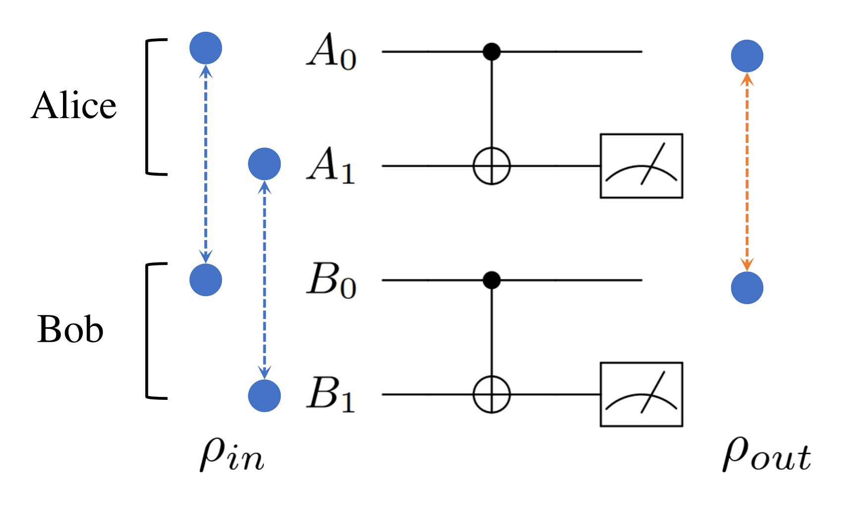
We have two remote parties, $A$ (Alice) and $B$ (Bob), involved in the BBPSSW distillation protocol. They share two qubit pairs $\rho_{A_0B_0}$ and $\rho_{A_1B_1}$. Each pair is initialized as $\rho_{in} = \rho_{\text{iso}}(p)$. These states could come from last distillation process or previously distributed and stored in some memory registers of a quantum network. Alice holds two qubits $A_0, A_1$, and Bob also holds two qubits $B_0, B_1$. With these initial setups, Alice and Bob implement the following LOCC process:
- Alice and Bob firstly choose the qubit pair they want to keep as the memory qubit pair to store entanglement resource after distillation. Here, they choose $A_0$ and $B_0$.
- Alice and Bob both apply a CNOT gate on their qubits. Here, they choose $A_0,B_0$ as the control qubits and $A_1,B_1$ as the target qubits.
- Two remote parties measure the target qubits then use classical communication channel to exchange their measurement results $m_{A_1}, m_{B_1}$.
- If the measurement results of Alice and Bob are the same (00 or 11), the distillation is successful, and the qubit pair $A_0, B_0$ is stored as state $\rho_{out}$; if the measurement results are different (01 or 10), they claim the distillation failed and the qubit pair $A_0, B_0$ will be discarded.
Note: The distillation protocol is probabilistic and it does not succeed every time. So, another metric to quantify the performance of distillation protocol is the probability of success $p_{succ}$. In general, there exists a trade off between the final state fidelity $F' = F(\rho_{out},\Phi^+)$ and $p_{succ}$. Theoretically, these two specific metrics for the BBPSSW protocol are provided as,
$$ F^{\prime}=\frac{F^2 + \frac{1}{9}(1-F)^2}{F^2 + \frac{2}{3}F(1-F) + \frac{5}{9}(1-F)^2}, \tag{10} $$where the initial fidelity $F(\rho_{in},\Phi^+) = (1+3p)/4$ with a probability of success,
$$ p_{\text {succ }}=F^{2} + \frac{2}{3}F(1-F) + \frac{5}{9}(1-F)^2. \tag{11} $$In the next section, we will go through how to simulate the BBPSSW protocol with Paddle Quantum.
Note: If the input state is not an isotropic state, one can depolarize it to an isotropic state with a twirling operation.
Simulation with Paddle Quantum
First, we need to import all the dependencies:
import numpy as np
from paddle_quantum.locc import LoccNet
import paddle
from paddle import matmul, trace
from paddle_quantum.state import bell_state, isotropic_state
from paddle_quantum.qinfo import logarithmic_negativity, is_ppt
For convenience, we introduce the metrics of BBPSSW here and later compare with the simulation result.
def BBPSSW_metrics(p):
    """
    Returns output fidelity and probability of success of the BBPSSW protocol.
    """
    F_in = (1+3*p)/4
    p_succ = F_in**2 + 2*F_in*(1-F_in)/3+ 5*(1-F_in)**2/9
    F_out = (F_in**2 + (1-F_in)**2/9)/p_succ

    return F_in, F_out, p_succ
In our example, the input state is an isotropic state with $p=0.7$, that is
$$ \rho_{in} = \rho_{\text{iso}}(0.7)= 0.7\lvert\Phi^+\rangle \langle\Phi^+\rvert + 0.075 I. \tag{12} $$p = 0.7
F_in, F_out, p_succ = BBPSSW_metrics(p)
print("The input fidelity is:", F_in)
print("The output fidelity is:", F_out)
print("With a probability of success:", p_succ)
print("The input state satisfies the PPT condition and hence not distillable?", is_ppt(isotropic_state(2, p)))
The input fidelity is: 0.7749999999999999
The output fidelity is: 0.8137583892617447
With a probability of success: 0.745
The input state satisfies the PPT condition and hence not distillable? False
Then we can simulate the BBPSSW protocol and check if the results match with theory.
class LOCC(LoccNet):
    def __init__(self):
        super(LOCC, self).__init__()
        # Add the first party Alice
        # The first parameter 2 stands for how many qubits A holds
        # The second parameter records the name of this party
        self.add_new_party(2, party_name='Alice')
        # Add the second party Bob
        # The first parameter 2 stands for how many qubits B holds
        # The second parameter records the name of this party
        self.add_new_party(2, party_name='Bob')

        # Define the input quantum states rho_in
        _state = isotropic_state(2, p)
        # ('Alice', 0) means Alice's first qubit A0
        # ('Bob', 0) means Bob's first qubit B0
        self.set_init_state(_state, [('Alice', 0), ('Bob', 0)])
        # ('Alice', 1) means Alice's second qubit A1
        # ('Bob', 1) means Bob's second qubit B1
        self.set_init_state(_state, [('Alice', 1), ('Bob', 1)])

        # Create Alice's local operations
        self.cir1 = self.create_ansatz('Alice')
        self.cir1.cnot([0, 1])
        # Create Bob's local operations
        self.cir2 = self.create_ansatz('Bob')
        self.cir2.cnot([0, 1])

    def BBPSSW(self):
        status = self.init_status
        # Run circuit
        status = self.cir1(status)
        status_mid = self.cir2(status)

        # ('Alice', 1) means measuring Alice's second qubit A1
        # ('Bob', 1) means measuring Bob's second qubit B1
        # ['00','11'] specifies the success condition for distillation
        # Means Alice and Bob both measure '00' or '11'
        status_mid = self.measure(status_mid, [('Alice', 1), ('Bob', 1)], ["00", "11"])

        # Trace out the measured qubits A1&B1
        # Leaving only Alice’s first qubit and Bob’s first qubit A0&B0 as the memory register
        status_fin = self.partial_state(status_mid, [('Alice', 0), ('Bob', 0)])

        return status_fin
# Run BBPSSW protocol
status_fin = LOCC().BBPSSW()

# Calculate fidelity
target_state = bell_state(2)
fidelity = 0
for status in status_fin:
    fidelity += paddle.real(trace(matmul(target_state.data, status.data)))
fidelity /= len(status_fin)

# Calculate success rate
suc_rate = sum([status.prob for status in status_fin])
fidelity_in, _, _ = BBPSSW_metrics(p)

# Output simulation results
print(f"The fidelity of the input quantum state is: {fidelity_in:.5f}")
print(f"The fidelity of the purified quantum state is: {fidelity.numpy()[0]:.5f}")
print(f"The probability of successful purification is: {suc_rate.numpy()[0]:#.3%}")

# Print the output state
rho_out = status_fin[0]
print("========================================================")
print(f"The output state is:\n {rho_out.data.numpy()}")
print(f"The initial logarithmic negativity is: {logarithmic_negativity(isotropic_state(2,p)).numpy()[0]}")
print(f"The final logarithmic negativity is: {logarithmic_negativity(rho_out).numpy()[0]}")
The fidelity of the input quantum state is: 0.77500
The fidelity of the purified quantum state is: 0.81376
The probability of successful purification is: 74.500%
========================================================
The output state is:
 [[0.48489934+0.j 0.        +0.j 0.        +0.j 0.32885906+0.j]
 [0.        +0.j 0.01510067+0.j 0.        +0.j 0.        +0.j]
 [0.        +0.j 0.        +0.j 0.01510067+0.j 0.        +0.j]
 [0.32885906+0.j 0.        +0.j 0.        +0.j 0.48489934+0.j]]
The initial logarithmic negativity is: 0.6322681307792664
The final logarithmic negativity is: 0.7026724219322205
Conclusion
As we can see, the simulation results matches the theoretical prediction perfectly. Through the BBPSSW protocol, we can extract an entangled state with a higher fidelity from two entangled states with low fidelities.
Advantages
- Operations are simple. Only CNOT gates are required.
- High success rate.
Disadvantages
- Strict requirements for the input state type. Isotropic states are preferred.
- Poor scalability. Unable to directly extend to the case of multiple copies.
We suggest interested readers to check the tutorial on how to design a new distillation protocol with LOCCNet.
References
[1] Chitambar, Eric, et al. "Everything you always wanted to know about LOCC (but were afraid to ask)." Communications in Mathematical Physics 328.1 (2014): 303-326.
[2] Bennett, Charles H., et al. "Purification of noisy entanglement and faithful teleportation via noisy channels." Physical Review Letters 76.5 (1996): 722.
[3] Bennett, Charles H., et al. "Teleporting an unknown quantum state via dual classical and Einstein-Podolsky-Rosen channels." Physical Review Letters 70.13 (1993): 1895.
[4] Bennett, Charles H., and Stephen J. Wiesner. "Communication via one-and two-particle operators on Einstein-Podolsky-Rosen states." Physical Review Letters 69.20 (1992): 2881.
[5] Ekert, Artur K. "Quantum cryptography based on Bell’s theorem." Physical Review Letters 67.6 (1991): 661.
[6] Życzkowski, Karol, et al. "Volume of the set of separable states." Physical Review A 58.2 (1998): 883.
[7] Peres, Asher. "Separability criterion for density matrices." Physical Review Letters 77.8 (1996): 1413.
[8] Gühne, Otfried, and Géza Tóth. "Entanglement detection." Physics Reports 474.1-6 (2009): 1-75.