Quantum Autoencoder¶

Copyright (c) 2021 Institute for Quantum Computing, Baidu Inc. All Rights Reserved.

Overview¶

This tutorial will show how to train a quantum autoencoder to compress and reconstruct a given quantum state (mixed state) [1].

Theory¶

The form of the quantum autoencoder is very similar to the classical autoencoder, which is composed of an encoder $E$ and a decoder $D$. For the input quantum state ${\rho }_{in}$ of the $N$ qubit system (here we use the density operator representation of quantum mechanics to describe the mixed state), first use the encoder $E=U\left(\theta \right)$ to encode information into some of the qubits in the system. This part of qubits is denoted by system $A$. After measuring and discarding the remaining qubits (this part is denoted by system $B$), we get the compressed quantum state ${\rho }_{encode}$! The dimension of the compressed quantum state is the same as the dimension of the quantum system $A$. Suppose we need $N_A$ qubits to describe the system $A$, then the dimension of the encoded quantum state ${\rho }_{encode}$ is $2^{N_A}\times 2^{N_A}$. Note that the mathematical operation corresponding to the measure-and-discard operation in this step is partial trace. The reader can intuitively treat it as the inverse operation of the tensor product $\otimes$.

Let us look at a specific example. Given a quantum state ${\rho }_A$ of $N_A$ qubits and another quantum state ${\rho }_B$ of $N_B$ qubits, the quantum state of the entire quantum system composed of subsystems $A$ and $B$ is ${\rho }_{AB}={\rho }_A\otimes {\rho }_B$, which is a state of $N=N_A+N_B$ qubits. Now we let the entire quantum system evolve under the action of the unitary matrix $U$ for some time to get a new quantum state $\widetilde{{\rho }_{AB}}=U{\rho }_{AB}{U}^{†}$. So if we only want to get the new quantum state $\widetilde{{\rho }_A}$ of quantum subsystem A at this time, what should we do? We simply measure the quantum subsystem $B$ and then discard it. This step of the operation is completed by partial trace $\widetilde{{\rho }_A}={\text{Tr}}_B\left(\widetilde{{\rho }_{AB}}\right)$. With Paddle Quantum, we can call the built-in function partial_trace(rho_AB, 2**N_A, 2**N_B, 2) to complete this operation. Note: The last parameter is 2, which means that we want to discard quantum system $B$.

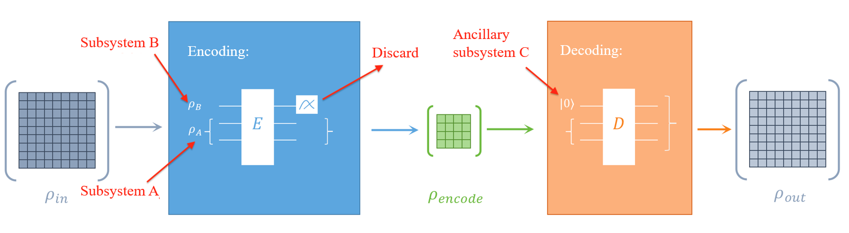
After discussing the encoding process, let us take a look at how decoding is done. To decode the quantum state ${\rho }_{encode}$, we need to introduce an ancillary system $C$ with the same dimension as the system $B$ and take its initial state as the $|0\dots 0⟩$ state. Then use the decoder $D=U^{†}\left(\theta \right)$ to act on the entire quantum system $A+C$ to decode the compressed information in system A. We hope that the final quantum state ${\rho }_{out}$ and ${\rho }_{in}$ are as similar as possible and use Uhlmann-Josza fidelity $F$ to measure the similarity between them.

$$\begin{array}{}F({\rho }_{in},{\rho }_{out})={\left(\mathrm{tr}\sqrt{\sqrt{{\rho }_{in}}{\rho }_{out}\sqrt{{\rho }_{in}}}\right)}^2.& \text{(1)}\end{array}$$

Finally, by optimizing the encoder's parameters, we can improve the fidelity of ${\rho }_{in}$ and ${\rho }_{out}$ as much as possible.

Paddle Quantum Implementation¶

Next, we will use a simple example to show the workflow of the quantum autoencoder. Here we first import the necessary packages.

Generating the initial state¶

Let us consider the quantum state ${\rho }_{in}$ of $N=3$ qubits. We first encode the information into the two qubits below (system $A$) through the encoder then measure and discard the first qubit (system $B$). Secondly, we introduce another qubit (the new reference system $C$) in state $|0⟩$ to replace the discarded qubit $B$. Finally, through the decoder, the compressed information in A is restored to ${\rho }_{out}$. Here, we assume that the initial state is a mixed state and the spectrum of ${\rho }_{in}$ is ${\lambda }_i\in \{0.4,0.2,0.2,0.1,0.1,0,0,0\}$, and then generate the initial state ${\rho }_{in}$ by applying a random unitary transformation.

Building a quantum neural network¶

Here, we use quantum neural networks (QNN) as encoders and decoders. Suppose system A has $N_A$ qubits, both system $B$ and $C$ have $N_B$ qubits, and the depth of the QNN is $D$. Encoder $E$ acts on the total system composed of systems A and B, and decoder $D$ acts on the total system composed of $A$ and $C$. In this example, $N_A=2$ and $N_B=1$.

Configuring the training model: loss function¶

Here, we define the loss function to be

$$\begin{array}{}Loss=1-⟨\mathrm{0...0}|{\rho }_{trash}|\mathrm{0...0}⟩,& \text{(2)}\end{array}$$

where ${\rho }_{trash}$ is the quantum state of the system $B$ discarded after encoding. Then we train the QNN through PaddlePaddle to minimize the loss function. If the loss function reaches 0, the input state and output state will be exactly the same state. This means that we have achieved compression and decompression perfectly, in which case the fidelity of the initial and final states is $F({\rho }_{in},{\rho }_{out})=1$.

If the dimension of system A is denoted by $d_A$, it is easy to prove that the maximum fidelity can be achieved by quantum autoencoder is the sum of $d_A$ largest eigenvalues ​​of ${\rho }_{in}$. In our case $d_A=4$ and the maximum fidelity is

$$\begin{array}{}{F}_{\text{max}}({\rho }_{in},{\rho }_{out})=\sum _{j=1}^{d_A}{\lambda }_j\left({\rho }_{in}\right)=0.4+0.2+0.2+0.1=\mathrm{0.9.}& \text{(3)}\end{array}$$

After 100 iterations, the fidelity achieved by the quantum autoencoder we trained reaches above 0.89, which is very close to the optimal value.

---

References¶

[1] Romero, J., Olson, J. P. & Aspuru-Guzik, A. Quantum autoencoders for efficient compression of quantum data. Quantum Sci. Technol. 2, 045001 (2017).